A remarkable range of phenomena of concern to researchers in many fields are often hierarchical (or nested) in nature. Patients are nested within doctors.Employees are nested within teams. Students are nested within classrooms (each of which has a different teacher), which are in turn nested within schools. In addition repeated measures are often captured such as in the case of daily diaries and ambulatory physiological measures taken a multiple times throughout a day over several days. In such cases, individuals measurements (i.e., observations) are clustered by day, which are in turn grouped by study participant. Whether they be of self-reports of thoughts and emotions or of physiological/behavioral indicators captured using ambulatory devices, multiple observations are recorded within a day, over a period of days across a sample of individuals.
The hierarchical nature of so much data has important implications for the analyses of such datasets. Consider an example where it is desirable to determine how well Grade 10 students are performing in Math at a particular school. There are 3 grade 10 classes at this school, each of which has a different teacher. A standard math test is administered to all students at the school and the scores tabulated. Of course there will be variance in scores across students — they are different people who may have studied to varying degrees, or who had varying degrees of pre-existing math proficiency and so on. But we would also expect that students within a class will more alike than students outside that class. In other words, the individual student Math scores are not independent — students in the same class will share variance — and this situation violates a key assumption of ordinary regression, which is that all observations be independent of each other.
Ordinary least squares regression, as well as most other widely used statistical tools, fail to take account of this non-independence of observations. If ordinary regression is nonetheless pursued, then hierarchical data must be “flattened” and the between-classroom variance is dumped together with the within-classroom variance into a single term, the error term. The big problem with this is that it will tend to produce inflated estimates of coefficients.
Multilevel modeling (MLM) is the statistical tool of choice to handle such situations in which the hierarchical nature of data means that there are multiple sources of variance. MLM enables each source of variance to be modeled separately, each in its own error term.
In the parlance of MLM, individual observations are at level 1. For example, every student’s math score would be at level 1. As students are grouped by classroom, the classroom (the grouping variable) would be considered level 2. In the case of diary studies and other real-time in situ designs involving repeated measures, each observation (such as a diary entry or glucose reading) would be at the level 1, and these would be grouped by study participant, which would be considered level 2.
In regression an equation is constructed such that an outcome variable is a function of a linear combination of predictor variables weighted by its own coefficient, which indexes how much a unit of change in the predictor is related to variation in the outcome variable. In ordinary (single-level) regression, the coefficients will be “fixed”. That is, the intercept and predictor coefficients will have only one value and they will be applied to all level 1 units regardless of the level 2 variables under which the level 1 unit is nested. In MLM, by contrast, there can be different intercepts and predictor coefficients for each level 2 unit. This is done by setting the coefficient that we wish to vary to random.
Perhaps one of the biggest issues with MLM is to decide whether an effect should be set as fixed or random. If there is a possibility, on theoretical or intuitive grounds, to expect that a slope or intercept should vary across higher into which the lower levels are grouped then these coefficients can be modeled as random. Typically the intercept is estimated as a random effect because this allows the means of level 1 units grouped under each level 2 unit to vary across level 2 units. In any event, a stepped procedure is typically performed in which the intercept is set to random and its fit tested against a model in which the intercept was set to fixed.
Random effects have both fixed and random components. The fixed effect is applicable to all level 1 units whereas the random component adjusts the fixed effect to a given level 2 unit, expressing the effect in terms of the deviation between the fixed effect component and the level 2 unit.
An Example
The following example uses a dataset from Hox (2010).
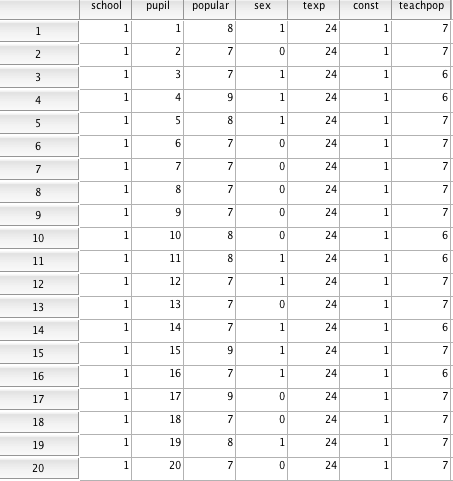
Suppose we have a dataset consisting of student popularity for a total of 2000 students from 100 classes. The table below shows the first 20 cases from this dataset. The outcome variable is popularity, which is a self-report rating on a scale from 0 (very unpopular) to 10 (very popular). Sex (0=boy, 1=girl) is the student level (level 1) predictor and teacher experience is a class level (level 2) predictor.
The first step in MLM analysis is to test a baseline or “null” model containing only a random intercept and no predictors. The aim is to test whether on average there is a difference in the outcome variable (popularity) across level 2 units (schools).
Although there are different frameworks for MLM modeling, it is helpful to use separate equations for each level.
Here are the 2 equations for a null model; that is, a model with no predictors. We have i level-1 observations are nested within j level-2 groups.
The first equation, Yij represents the outcome variable (in this case, popularity), β0j represents the mean popularity across all of school j‘s students, and rij represents the difference between school j‘s mean popularity and the popularity of student i.
![]()
![]()
In the second equation, γ00 represents the grand mean (the average popularity computed across all schools), and μ0j represents the difference between school js average and the grand mean. The inclusion of the μ0j term signals that we wish to model the intercept as random. And indeed, that we use separate equations for each level makes it easy to see which coefficients are modeled as fixed and which as random. The equation indicates that there is both a fixed component (γ00) and a random component (μ0j).
We can, however, write out the full equation by substituting the level 2 equation into the level 1 equation, which gives us:
![]()
This equation makes it easy to see that the popularity of student i in school j is a function of 3 components: how average popularity of students across all students, plus how much school j deviates from this grand mean, plus how much student i‘s popularity deviates from school j‘s average. So the variance terms μ0j and rij correct the prediction according to the two sources of variance: 1) how much a school deviates from the mean of all schools and 2) how much a student deviates from the mean within a school.
So let’s run the mixed model analysis in SPSS. Following is a portion of the output:

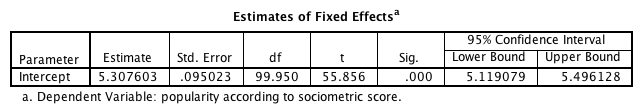

We can see that the fixed component of the effect, (γ00) is 5.308. This means that on average, schools had a student popularity of about 5.31, which is shown to be statistically different from 0, t(100) = 55.86, p < .001. But the question is: did schools differ as to the average popularity of their students. In essence, what we are testing is whether the variance of the random component is significantly different from 0. The variance of the random component is denoted by τ00 and residuals are denoted by σ2.
If there is little difference from from one school to the other on average student popularity then the variance across schools should be minimal or not at all. As can be seen in the Estimates of Covariance Parameters table above, the variance across all j schools (the μ0j’s) is τ00 = .871, which, according to the Wald Z test, is is statistically different from 0, Z = 6.817, p < .001.
An alternative to the Wald Z test is to compare the deviances of both the random intercept model and the baseline (null) model: one in which an effect is allowed to vary (random) across the higher level units and one in which the effect is fixed. We use a likelihood ratio test, which provides a way to assess how many times more likely the data are under one model compared to another.
To perform this comparison, let’s run a null model by eliminating the random component.
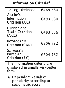
The difference between the two is 6489.53 – 5112.722 = 1376.808. The difference in these log likelihood values is distributed as chi-square. As the models differ by one parameter (the random component) there is 1 df. So chi-square (1) = 1376.808, p<.001. Therefore we can reject the null hypothesis that the variance of the random intercepts components is 0.
It is possible to estimate the degree to which an values on an outcome variable between level 1 units are correlated or independent of each other. The measure is the Interclass Correlation Coefficient (ICC). If they are not independent then there is probably no need to model a relationship as random.
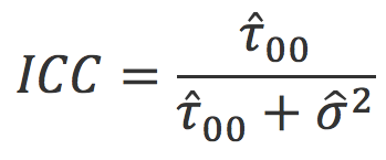
From the SPSS output above we can see that τ00 = .871 σ2 = .639.

This can be interpreted as follows: About 58% of the total variance popularity scores is accounted for by differences in schools. In other words, school makes a difference. The higher the ICC score is, the greater the dependance on groupings in the outcome values and hence the greater the suggested need for a random component to the model.
Well that pretty much does it for the first part of my MLM primer. Up next we will see what happens when adding a predictor to the model. In particular, would sex add anything to the predictive power of our model. Please look out for Part 2.
Data
Example data available through http://www.ats.ucla.edu/stat/hlm/examples/ma_hox/default.htm.
References
Hox, J (2010). Multilevel Analysis: Techniques and Applications, Second Edition. Routledge, NY.
