Purpose
Logistic regression (LR) is a statistical tool that permits the examination of the relationship between one or more predictor variables (e.g., weight, age, average daily exercise) and a categorical outcome variable (survival, presence of disease, success. It is used for 2 primary purposes: 1) Explanation and 2) Prediction.
Explanation aims to identify which variables are associated with significant changes in the odds of some event occurring. For example, we may wish to know which from among a set of factors (e.g., sex, length of time in pain, stress levels) change the odds of development of a chronic pain condition. In this case the interest is in gaining a better understanding of the mechanisms involved.
Prediction aims to predict to which group individual cases are most likely to belong. For example, we may wish to know what is the likelihood that individuals with a given set of characteristics (e.g., age, sex, SES) will purchase a product. In this case, the interest is not so much understanding mechanisms as with how well some outcome can be predicted.
| Similarity Betweeen Logistic and Multiple Regression |
| Logistic regression is similar to multiple regression (MR) in that the goal is to model the relationship between a set of variables and some outcome and to predict the outcome based upon this set of variables. Thus, they are both very useful in that they can be used to both understand how variables are related and for making predictions |
| Difference Between Logistic and Multiple Regression |
| The difference between logistic and multiple regression has to do with the nature of the outcome variable. in the case of LR, the outcome variable is categorical (e.g., survived/died, succeeded/failed, purchased/didn’t purchase, etc.), whereas in the case of MR, the outcome variable is continuous (e.g., pain rating, glucose level, product satisfaction rating, etc.). |
Some Applications
The applications of logistic regression are many. Among numerous other things, LR models can be generated that can be used to predict…
- The risk of adverse cardiac event occurring from variables such as age, blood pressure, cholesterol level, and weight.
- The likelihood that a customer will subscribe to a service based on sex, household income, education level, and previous purchase history.
- The probability that post-surgical patients will develop chronic pain based on history of stress, anxiety and other psychological factors.
- Whether or not a customer will re-visit a store or event based on a set of feedback data collected in previous years.
- To understand which customers are most likely to stay (and which to leave) based on a host of demographics, feedback, and social media data.
Logistic Regression Process
The LR analysis process typically proceeds as follows:
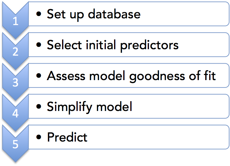
Step 1: Set up a dataset consisting of a sample of cases. Columns should contain data for the predictor variables and the outcome variable, and each row should contain a separate individual case. Categorical predictors will need to be coded so that numbers represent categories. Dummy coding is the most common method of coding. Statistical software (e.g., SPSS) may perform this coding automatically. The outcome variable should be coded so that numbers represent group membership (e.g., 1 = failure, 2 = success).
Step 2: After the dataset is organized into a table per step 1, the next step is to select the initial set of predictors to include in the LR model. The identification of these variables can be theory driven, based on previous research, or exploratory. For example, it may be known that family history of cardiovascular disease is a significant predictor of whether an individual will experience an adverse cardiac event, but investigators may wish to know whether adding level of chronic stress might significantly increase the predictive power in the model.
Step 3: After the data have been prepared and coded, and the initial set of predictors identified, it is possible to run the LR analysis using statistical software (e.g., SPSS, SAS). The first question will be whether there is an overall relationship between the set of predictors and the outcome. The analysis, and model generation, is performed on a dataset in which the outcome is known.
For example, can knowing about age, sex, family history of condition, and level of chronic stress predict onset of a particular disease? To answer this question an LR analysis would be performed on a data set containing a sample of cases in which data are provided for the predictors and whether or not each case contracted the disease. In a sense, the LR procedure will use these data to “learn” about how the predictors and outcomes are related.
To assess how well the model fits the data (i.e., its goodness-of-fit.), the full model with a set of predictor variables is compared against a baseline model, in which the predictors have been omitted. We will see exactly how this is done later.
Step 4: Assuming the model provides a good fit (ie., it fits the data significantly better than a baseline model with no predictors), the next step is to determine which of the included variables are significant independent predictors of the outcome. The aim here is to develop the simplest possible model by including only those predictor variables that improve the predictive power of the model.
For example, does including chronic stress improve the model’s ability to predict who will contract an illness? This is typically accomplished by examining whether the predictor coefficients are statistically significant, or by testing whether the elimination of a predictor harms how well the model fits the data.
Just as in multiple regression, LR models can include interaction terms. For example, family history of a disease may only predict disease onset in the context of high chronic life stress. Among interactions between continuous variables (e.g., stress level and pain rating), centering the variables can avoid potential multicollinearity.
An important question is just how strong is the relationship between the set of predictors and the outcome in a model? What proportion of the variance in the outcome is explained by the set of predictors?
Step 5: In the final step, assuming a satisfactory goodness-of-fit, the model can be used to predict new cases. Values for the predictors are entered into the regression equation, which results in the odds that a case would fit into a particular category. Results are typically expressed in terms of Odds Ratios. An odds ratio expresses the ratio of the odds that an event will occur to the odds that the event will not occur.
| Facts about logistic regression |
|
Background
You may remember that in multiple regression (MR), an outcome variable Y is predicted based upon a linear combination of one to many predictor variables multiplied by a weight (regression coefficient):
![]()
In this case, Yi is a continuous variable and a precise value is predicted based upon a set of values provided for each of the predictor variables X1…n. With logistic regression, on the other hand, the outcome variable is discrete and we predict the probability of each discrete outcome:
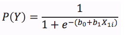
In this equation P(Y) is the probability that some outcome category will occur, such as the probability of success or a sale or death.
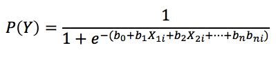
If you look closely at the equation you will probably notice that it incorporates the same linear combination of weighted predictors as in simple linear regression. It can be extended to include any number of predictors, just as in MR:
So why can’t we just use MR? The reason is primarily because the assumption of linearity is violated when the outcome variable is categorical. So how can we turn a non-linear relationship into a linear one so that it can be attacked using a regression model? Simple. Use a logarithmic transformation. Logistic regression converts a non-linear regression model into logarithmic terms.
The goal of analysis is to estimate the set of regression coefficients for each of the predictors included in the model such that the model best fits the observed data.
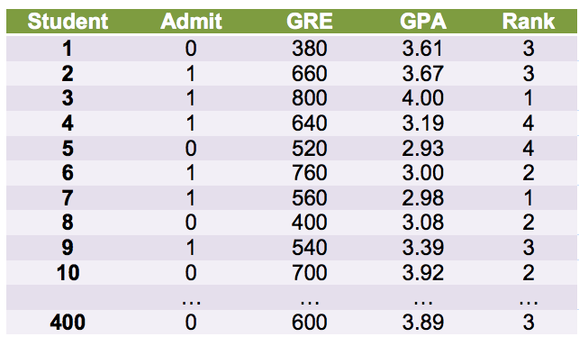
Before getting any more embroiled in the details, let’s look at a simple example. The data for this example come from the UCLA statistical service[1].
In the example, a set of data on 3 predictor variables (GRE scores, GPA, school ranking), and an outcome variable (whether they had been admitted to graduate school or not) have been collected from 400 students. The goal is to generate a logistic regression model that can be used to predict whether or not a given individual student will be admitted based on values on the 3 predictors for this given student. The following table contains the first 10 and last case of the 400.
I will next run the binary logistic regression analysis in SPSS.
Step 1: Set up dataset
For this example the dataset has been prepared. Therefore we can assume that Step 1 in the LR process has been performed.
Step 2: Select predictors
In this example, a set of predictors has already been chosen. Their selection was probably based upon anecdotal or experiential reports. Therefore we can assume that Step 2 in the LR process has been performed.
Step 3: Goodness of fit?
The dataset has been cleaned and prepared, and the initial set of predictors has been selected. The question now is, does a relationship exist between the 3 predictors (GRE, GPA, Rank), and outcome (Admit/No-Admit)? To answer this question, it is necessary to compare a model containing the predictors against a baseline model containing only the constant.
Let’s go ahead and use SPSS to perform an LR analysis. To do so, access the Logistic Regression module by going to the Analyze menu and selecting Regression >> Binary Logistic… This will display a dialog box that looks like this…

Three decisions must be made in the Logistic Regression dialog box: 1) variables to include, 2) how to code categorical variables, and 3) method of variable entry.
First, the outcome variable, Admit (whether or not a student was admitted to graduate school) is moved to the Dependent box and the predictors are moved to the Covariates box.
Second, the coding for the categorical variable, Rank, is specified in the “Define Categorical Variables” dialog box, which is obtained by clicking the “Categorical…” button. I have chosen “Indicator” coding.

Third, method of entry is specified using the drop-down menu. As in Regression, the Enter method, in which all predictors are entered simultaneously, is the most common and typically most appropriate method.
After specifying these 3 pieces of information in the Logistic Regression dialog box and clicking the “OK” button, the results are produced.
As mentioned earlier, SPSS automatically codes any variables specified as categorical. The table, Categorical Variables Codings, shows how each of the 4 values in the variable Rank was coded and the frequency of occurrence for each. It appears that schools ranking 2 were the most frequent (151), with those scoring 1 appearing the least frequently (61).
| Categorical Variables Codings | |||||
| Frequency | Parameter coding | ||||
| (1) | (2) | (3) | |||
| rank | 1 | 61 | 1.000 | .000 | .000 |
| 2 | 151 | .000 | 1.000 | .000 | |
| 3 | 121 | .000 | .000 | 1.000 | |
| 4 | 67 | .000 | .000 | .000 | |
Ascertaining how well the model fits the sample data entails 3 steps: 1) assess the goodness-of-fit of the basic model, with no predictors, 2) assess the goodness of fit of the full model, with all predictors entered, and 3) determine whether the difference in goodness of fit indices between the two models is statistically significant. Thus we compare the fit of the model with all predictors against one without any predictors. The fit of a model is quantified by computing the Log-Likelihood. Likelihood in statistics refers to the likelihood that a particular population would produce the data observed in the sample. The classic example is of a coin that results in a heads up 10 times in a row. What is the likelihood that such an outcome would be produced by a fair coin? Applied to logistic regression, it would be the likelihood that the population of students would produce the data observed in the sample. In LR we use the log-likelihood function:
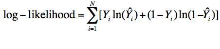
To determine goodness-of-fit of the model, the log-likelihood (LL) of both the baseline and full models are computed. Then the LL of the base model (smaller) is subtracted from the full model (bigger), producing a chi-square value, as in the following equation:where is the estimated probability of a given outcome for the ith case.
![]()
After chi-square is calculated its significance is tested using the difference in degrees of freedom between the bigger and smaller models. The equation expresses the models in terms of bigger and smaller because any two models can be compared assuming that they are hierarchical such that all elements of the smaller model are incorporated into the bigger model.
![]()
The Iteration History table shows the log-likelihood of the baseline model.Let’s look at how this plays out in SPSS. The analysis begins with “Block 0”, which is the baseline model. In this model all of the predictors are omitted, leaving only the constant.
| Iteration Historya,b,c | |||
| Iteration | -2 Log likelihood | Coefficients | |
| Constant | |||
| Step 0 | 1 | 500.085 | -.730 |
| 2 | 499.977 | -.765 | |
| 3 | 499.977 | -.765 | |
|
|||
For the baseline model, in which only the constant is included, SPSS assesses the model by assigning everyone to a single category. In this case it would be to either “Admit” or “No Admit”. The category it chooses is simply the one that will lead to the greatest number of cases being correctly predicted. In our example, given no additional information, it is best to simply predict “No Admit” because this yields 273 correct classifications out of 400, whereas predicting “Admit” would produce a considerably less impressive 127 correct classifications out of 400. As the Classification Table reveals, this produces a 68% overall accuracy.
| Classification Tablea,b | |||||
| Observed | Predicted | ||||
| admit | Percentage Correct | ||||
| No Admit | Admit | ||||
| Step 0 | admit | No Admit | 273 | 0 | 100.0 |
| Admit | 127 | 0 | .0 | ||
| Overall Percentage | 68.3 | ||||
|
|||||
The Variables not in the Equation table is useful in that it provides residual chi-square statistics (Overall Statistics), indicating whether the inclusion of these variables in the model will significantly improve its predictive power. In this case, the score is 40.16, which is significant at p < .001.
| Variables not in the Equation | |||||
| Score | df | Sig. | |||
| Step 0 | Variables | gre | 13.606 | 1 | .000 |
| gpa | 12.704 | 1 | .000 | ||
| rank | 25.242 | 3 | .000 | ||
| rank(1) | 16.590 | 1 | .000 | ||
| rank(2) | 1.801 | 1 | .180 | ||
| rank(3) | 5.934 | 1 | .015 | ||
| Overall Statistics | 40.160 | 5 | .000 | ||
In the next step, the predictor variables are entered by SPSS into the model and tests to what degree this new model predicts outcome classifications better than the baseline model.
When only the constant was included, the -2LL value was 499.98. With the inclusion of the predictor variables, the -2LL value in the Model Summary table has changed to 458.52, a drop of 41.46. This drop would appear to indicate that the inclusion of GPA, GRE and Rank improve the model’s ability to accurately predict admission status. The question remains, however, as to whether this difference reflects a true difference in the population. As the difference in -2LL values between models has a chi-square distribution, it is possible to determine its significance. As indicated in the Omnibus Tests of Model Coefficients table, the chi-square value of 41.46, with 5 df (number of parameters in new model + 1 subtract number of parameters in the baseline model), is significant at p < .001. This test can be considered analogous to the F-test in multiple regression.
| Omnibus Tests of Model Coefficients | ||||
| Chi-square | df | Sig. | ||
| Step 1 | Step | 41.459 | 5 | .000 |
| Block | 41.459 | 5 | .000 | |
| Model | 41.459 | 5 | .000 | |
| Model Summary | |||
| Step | -2 Log likelihood | Cox & Snell R Square | Nagelkerke R Square |
| 1 | 458.517a | .098 | .138 |
|
|||
The inclusion of the 3 predictors has improved overall accuracy of our predictions from 68% to 71%. Whether this improvement is meaningful or important depends on the particular domain and the purpose to which the model will be applied.
| Classification Tablea | |||||
| Observed | Predicted | ||||
| admit | Percentage Correct | ||||
| No Admit | Admit | ||||
| Step 1 | admit | No Admit | 254 | 19 | 93.0 |
| Admit | 97 | 30 | 23.6 | ||
| Overall Percentage | 71.0 | ||||
|
|||||
The Variables in the Equation table shows the estimates for the coefficients for the predictors included in the model. These coefficients can be interpreted similarly to their linear regression counterparts. They indicate the change in the natural logarithm of the odds (i.e., the logit) of an event occurring for every one-unit change in the predictor variable. The Wald statistic reveals whether the coefficient is significantly different from 0.
| Variables in the Equation | |||||||||
| B | S.E. | Wald | df | Sig. | Exp(B) | 95% C.I.for EXP(B) | |||
| Lower | Upper | ||||||||
| Step 1a | gre | .002 | .001 | 4.284 | 1 | .038 | 1.002 | 1.000 | 1.004 |
| gpa | .804 | .332 | 5.872 | 1 | .015 | 2.235 | 1.166 | 4.282 | |
| rank | 20.895 | 3 | .000 | ||||||
| rank(1) | 1.551 | .418 | 13.787 | 1 | .000 | 4.718 | 2.080 | 10.702 | |
| rank(2) | .876 | .367 | 5.706 | 1 | .017 | 2.401 | 1.170 | 4.927 | |
| rank(3) | .211 | .393 | .289 | 1 | .591 | 1.235 | .572 | 2.668 | |
| Constant | -5.541 | 1.138 | 23.709 | 1 | .000 | .004 | |||
|
|||||||||
It is possible to see that for every one-unit change in GRE, the logit (log odds) of admission (vs non-admission) increases by 0.002, and for every one-unit increase in GPA, the log odds of being admitted increases by 0.804.
As Rank is a categorical variable it must be interpreted differently. The coding for the variable specified that the last value (i.e., 4) be treated as the reference category. Thus attending a university with a rank of 1 compared to a university with rank 4 improves log odds of admission by 1.56.
By exponentiating the b values, they can be interpreted as odds ratios. SPSS performs this computation and the results are listed in the Exp(B) column in the Variables in the Equation table. It is apparent that for every one unit increase in GPA, the odds of being admitted to graduate school (versus not being admitted) increase by a factor of 2.23, and for every one unit increase in GRE scores, the odds of being admitted remain about the same (odds ratio = 1). Being in a top ranking school compared to the lowest ranking school will increase the odds of admission by as much as 4.72.
An odds ratio greater than 1 means that as values in a predictor increase so to the odds of an outcome increase. An odds ratio less than 1 indicates that the as as predictor values increase, the odds of the outcome occurring decrease.
Note that the confidence interval of Exp(B) values can be examined to see whether it crosses 1. As long as the interval is full above or below 1, you can be confident at the 95% level that the direction of the odds ratio value estimate (above or below 1) reflects that in the population.
And that’s your friendly primer on Logistic Regression.
