Linear regression (MR) may just be the single most useful and widely applicable statistical tool available.
Purpose
LR is a statistical technique that enables us to investigation the relationship between some set of variables (e.g., weight, age, average daily exercise) and some outcome (e.g. level of fatigue reported). It can be used for 2 primary purposes: 1) Explanation and 2) Prediction.
Explanation refers to the ability to determine which variables explain variance in some outcome variable. For example, we may wish to know which from among a set of factors (e.g., sex, length of time in pain, stress levels) explain the variance in pain relief given administration of a particular drug and what proportion of this variance is explained by those factors. In this case, the interest would be to gain a better understanding of the mechanisms involved.
Prediction refers to the ability to predict the value of an outcome variable based on some set of predictor variables. For example, we may wish to know what is the likelihood that individuals with a given set of characteristics (e.g., age, sex, SES) will purchase a product. In this case, the interest would be to develop a model that would make the best possible predictions.
Regression is remarkably flexible and powerful. It can be used to explore the following:
- how much of the variance in your outcome variable can be explained by all of the independent (predictor) variables,
- the predictive power of each of the predictor variables while controlling for all the other predictors in the model,
- the relative predictive power among predictors,
- any of the predictors interact with other predictors.
Typically regression is implemented with multiple predictors, although only a single predictor is necessary. The former type is called Multiple Regression, while the latter is referred to as Simple Regression.
Example
Let’s take a look at a simple example to see how regression analysis works. The following table lists the age, weight and systolic blood pressure measures for 10 individuals.
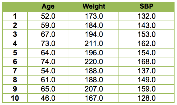
Say that the goal is one of prediction. In particular we want to know whether it is possible to predict someone’s weight given his or her age. As this example entails a single predictor (i.e., age), it is an example of simple regression. On the basis of personal observations, we might hypothesize that as people get older their weight tends to increase.
The first step should be to plot the data on a scatterplot to get a sense for how the data look. On the graph below I’ve done just that. Each of the 10 circles represents a single individual’s values on both Age and Weight.

A general trend in which higher age predicts greater weight is evident from the graph. It appears, therefore, that our hypothesis is correct. But this is just a sample of data taken from 10 individuals. In general, the concern is not with a sample per se. Instead the aim is almost always to extract some general knowledge about the population from which the sample was taken. We want to be able to generalize the findings to the population. So what we would really need is to build a model of the relationship between age and weight in the population based upon the sample. With such a model in hand it would be possible to predict someone’s weight given their age as long as that person is a member of the population from which the sample was randomly drawn.
Regression models provide a way to do just that. What does a regression model look like? It is simply a mathematical equation that can be shown to represent points of data as accurately as possible, minimizing the error between prediction and actual data points. Almost any kind of relationship among variables from simple linear associations to highly complex non-linear relationships can be modeled.
Examining the plot of Age and Weight it is easy to see that the data points fall on more or less a straight line. Therefore an equation of a straight line seems the right kind of regression model. Thus, we can represent (i.e., model) a set of data with a straight line.
You may remember that the equation for a straight line is:

where Y is the outcome variable (weight in our example), X is the predictor variable (age in our example) and a and b represent the Y-intercept and slope of the line, respectively.
The goal is to generate a line that has the intercept and slopes that best fit the data points in the sample. We could eyeball the data and draw a line that looks like a good fit, but that would be inexact and would be unlikely to yield the line that best fits the data observed.
It turns out that there is a method of fitting the best line to the data. The method is called the method of least squares. As you can see in the figure below, this method finds a line such that the difference between the line and the data points from which the line was based is minimized. The differences between the line and data points are called residuals and are represented by the red dotted lines in the graph. So the goal with regression is to compute the line that minimizes the sum of all these residuals. Actually, if you were to add up all these differences you would wind up with 0. So to avoid this, each of the differences is squared (to eliminate the negative signs) and using that technique you wind up with the sum of squared differences or the sum of squares.

Ok, so this line represents the best fit to the data. But just how good of a fit is it? In other words, what is the goodness of fit of the model?
The strategy that is typically used is to compare the regression model with the mean.
Let’s return to the formula for a straight line (eq 1). The b in the equation is the slope of the line. In the context of Regression it is referred to as a regression coefficient. It is the amount of change in Y (in this case, weight) for every unit change in X (in this case, age). The regression coefficient quantifies the relationship between X and Y.
The a in the equation is called the y-intercept, and represents the value of Y when X is 0. Think about what this means. Considering our example, say there is no information available about age, you are given a particular individual and asked for your best guess as to what this individual’s weight is. What would your best guess be? Well, in general, if you are asked to predict a value on some variable and you have no other information than a sample of data for that variable, you would be best to predict the mean value for that variable. If armed only with temperature for Oct 15 for the past 10 years and you what will be the temperature this coming Oct 15, your best guess would be the mean temperature from past years. If supplied with exam score of every student in a class and are asked how Sally did, your best guess would be the mean exam score for the class.
Thus, if there is no information about the variable X, and therefore remove it from the equation (which is achieved by plugging in 0 for X), then your best prediction essentially becomes a, the y-intercept. The y-intercept is the mean of Y. Thus, in the absence of any information regarding the relationship between X and Y, the best prediction will simply be the mean of Y. I find it helpful to call this the baseline model.
The goodness of fit, therefore, can be calculated based upon how much better it helps us to predict Y over and above the mean of Y (the baseline model), which is our best prediction in the absence of any further information regarding the relationship between X and Y.
The next question then is how can this “how much better” it predicts the outcome be quantified? The answer involves the residuals again.
The first quantity we need to know is the total amount of variation there is in the outcome variable. As you may know, in statistics, variation is typically expressed in terms of the amount of spread in data about the mean.
This quantity is known as the total sum of squares (SSTOT). SSTOT is a measure of the total variation, and is calculated as the sum of the squared deviations of the outcome variable from its mean:

SSTOT is represented by the difference between each point and the mean:

Whereas SSTOT is an index of total variance, SSMOD represents the difference between points on the model line (the line representing the regression equation) and the mean. This is visible in the Figure below:

To arrive at this figure, we calculate the differences between the observed values and the values predicted by the line of best fit model. That will give the residual sum of squares (SSR). If we subtract SSRES from SSTOT then we will be left with the portion of the total SS, SSMOD, that is uniquely predicted by the regression model over and above the basic model, the mean.

To obtain an measure of much of the variance in the outcome Y (weight in the example) is explained by the model (SSMOD) relative to the total amount of variance to be explained (SSTOT), we compute R2, the coefficient of determination.

R2 can be any value between 0 and 100. An R2 of 0 means that the predictor variables explain none of the variance in the outcome variable, and an R2 of 100 means that variation in the outcome variable is entirely explained by the predictor variables. Of course these extremes seldom occur.
To ascertain whether R2 is statistically significant, it is possible to calculate an F-statistic. The F-statistic is computed based on the ratio of SSMOD and SSRES. For the F-statistic we actually use the mean sum of squares (or mean squares).


So F is an index of the degree to which the model as a whole has improved the ability to predict the outcome variable when held up agains the residuals (the diff between predicted and observed values). Because it is an F distribution, it’s statistical significance can be tested.
But what about the individual predictors?
Returning to the Eq 1, the equation for a straight line, b is the coefficient representing the slope of the line. The slope tells us by how much Y increases for every unit increase in X. In our example, it would be how much weight increases for every year increase in age. What if there was absolutely no relationship between age and weight? The line would be flat. That’s because weight would not increase at all for each unit increase in age. A flat line has a slope of 0. So to determine whether a b-coefficient is significant, we use a t-test to determine the degree to which b is significantly different from 0.
To do so, the t-test essentially assesses whether b is big relative to the amount of error inherent in that estimate.

The computed t is then compared against a critical value such that it would be 5% or less likely to have occurred by chance using N-p-1 degrees of freedom where N is the total sample size and p is the number of predictors.
Let’s run the age-weight data through the Linear Regression function in SPSS. The Model Summary table provides information relating to the fit of the model.
| Model Summary | ||||
| Model | R | R Square | Adjusted R Square | Std. Error of the Estimate |
| 1 | .940a | .884 | .870 | 5.973 |
|
||||
In particular it provides R and R2. When there is only one predictor, R is the simple correlation between the predictor (age) and the outcome (weight). R2, the square of R, can be interpreted as the percentage of the outcome variable (weight) accounted for by (or “explained by”) age. In this example, 88% of the variation in weight is accounted for by our single predictor, age.
The next table is the ANOVA table:
| ANOVAa | ||||||
| Model | Sum of Squares | df | Mean Square | F | Sig. | |
| 1 | Regression | 2180.211 | 1 | 2180.211 | 61.115 | .000b |
| Residual | 285.389 | 8 | 35.674 | |||
| Total | 2465.600 | 9 | ||||
|
||||||
ANOVA tells us whether the overall model provides a significant amount of improvement in prediction of the outcome variable (weight). This table provides the SSM, SSR, and SST, MSM and MSR. As indicated above, the formula for F is:

We can see that p < .001, meaning that there is less than a .1% chance that this F value would have occurred by chance alone, that is that we would erroneously reject the null hypothesis when it is in fact true. Put another way, it is the likelihood of a false alarm, concluding that the model predicts a significantly greater amount of the variance in weight relative to the model based on the mean (SSTOT).
The next table provides the significance of the individual model parameters. In the case of this simple regression example in which there is a single predictor only, the only parameters are the constant and age:
| Coefficientsa | ||||||
| Model | Unstandardized Coefficients | Standardized Coefficients | t | Sig. | ||
| B | Std. Error | Beta | ||||
| 1 | (Constant) | 86.554 | 13.721 | 6.308 | .000 | |
| age | 1.728 | .221 | .940 | 7.818 | .000 | |
|
||||||
B0 is the intercept, the value of Y when X=0. In the SPSS Coefficients table, the (Constant) is the y-intercept value, 86.55. The coefficient b1, the slope, is estimated to be 1.73. Therefore for 1 unit increase in age, weight increases by about 1.73 pounds, a change that is highly significant at p < .001.
So there you have it, my primer on linear regression. Although the example here contained only a single predictor, in almost all real-world applications of regression there will be multiple predictors and hence you will be performing multiple regression. It is important, however, to understand the basics of regression before tackling multiple regression, a topic to which I will turn in another article.
