A test of significance amounts to a question as to whether the effects observed in a sample reflect a true effect in the population from which the sample was drawn. To answer this question, we use a strategy. We assess the probability that the effect observed in the sample would have occurred by chance given that the null hypothesis (that there are no differences) is true. Thus in essence a test of statistical significance amounts to an assessment the likelihood that an observed effect would have occurred by chance. To do this, we use compare our results against a known distribution. When our data are continuous we can use calculate a z-score and compare our results against the normal distribution. If we have a small sample size we can use calculate a t-score and compare this score against the t-distribution.
These are appropriate tests when the data are continuous but not when they are categorical. The chi-square distribution is used where the data are categorical. While the normal distribution has 2 parameters, the mean and standard deviation, the chi-square distribution has only one parameter, k, representing the degrees of freedom. And just as one can plot different normal curves based on different means and standard deviations, one can plot different chi-square curves based on different degrees of freedom.

1 df

2 df

3 df
Chi-Square Goodness of Fit Test
Categorical data are measured in terms of whether an individual case belongs or does not belong to a particular category. Variables measured on a continuous scale (e.g., age, intensity of pain, interest level) can be summarized in terms of means and medians. These measured do not make sense in the case of categorical variables, which are instead summarized as frequencies.
The chi-square goodness of fit test provides a way to assess the probability that the observed frequencies differ from the expected frequencies, which are the category frequencies that would be expected by chance.
Say you want to know whether blood types from a random sample of surgical patients conforms to the distribution of blood types in the general population. The frequency distribution of blood types taken from the same are the observed frequencies. The frequency distribution of blood types in the population are the expected frequencies. It is easy to see that obtaining frequencies in our sample that look a lot like the frequency distribution in the population would suggest that our sample frequency distribution does not differ from what would be expected by chance.
The table below presents the data obtained from a sample of 173 surgical patients summarized as frequencies.
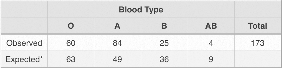
The next step is to obtain a chi-square statistic. The equation is as follows:

Substituting the numbers from the table into the equation, we get:

Now that we have the chi-square statistic we must next compare it to the chi-square distribution in order to determine the probability of a chi-square value this extreme given that the null hypothesis is true.
If you were running a chi-square analysis in a statistical app then it would provide this probability value in its output. However it is also possible to set a particular probability level (most commonly .05 or .01) and look up the critical value of chi-square for which a chi-square statistic above which we can reject the null hypothesis that our observed distribution follows a chance distribution. We can use a table similar to the figure below to look up this critical value. All we need is the p-level and the degrees of freedom.
For our example we have k-1 df where k is the number of categories. So to obtain the critical ch-square value find the column with the p-level we wish to use (in this case .05) and find the row with the correct degrees of freedom (in this case 3). So our critical chi-square value is
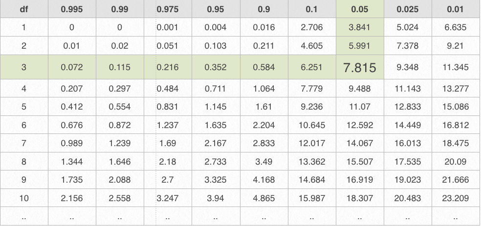
Given that the X2 statistic that we computed, 31.28, is greatly exceeds X2 critical we can safely reject the null hypothesis and conclude that the expected frequencies differed from those that would be expected by chance. For whatever reason, this particular sample of surgical patients have a blood type distribution that is significantly different from those expected given the distribution in the population.
Decomposing the significant result
A significant chi-square means that the variables are unlikely to be independent in the population. But what is driving this result? It is possible for some cells to deviate significantly from expectation whereas others do not.
To decompose the overall chi-square test, we can look at the residuals for each cell; that is, the amount by which an observed count deviates from the expected count for each cell. By then standardizing the residuals we essentially turn them into z-scores and once they are in the form of z-scores their significance can be easily assessed. Here is the formula:

Given that each standardized residual is a expressed as a z-score we can easily determine its statistical significance.
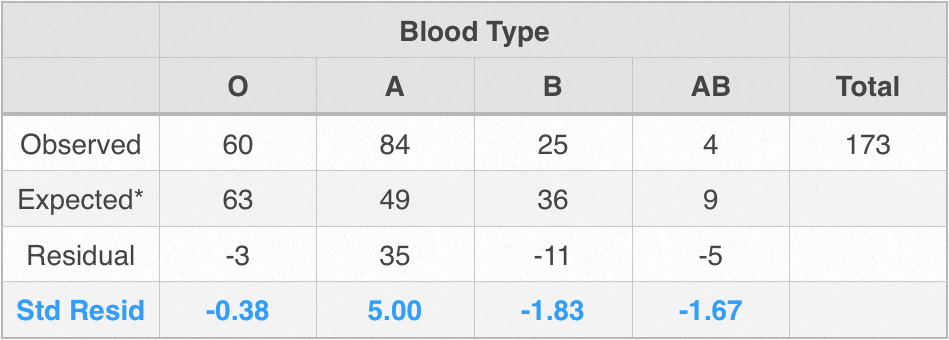
Using the formula above, standardized residuals were calculated for the 4 blood types and are presented in the final row of the table above.
On a normal distribution, we know that 95% of all values will be found within 1.96 standard deviations of the mean. That means that a z-score would have to be greater than +/- 1.96 for it to exceed a 5% chance that it has occurred by chance. Only standardized residual for blood type A, 5.00, exceeds 1.96. Therefore the significant chi-square result was driven by the fact that in this sample, there was a far greater number of pre-surgical patients with type A blood than would be expected by chance but that observed frequencies for the other blood types were within chance levels.
Test of independence
The chi-square test of independence is appropriate when you have 2 categorical variables and the total number of individual cases in your sample are distributed among the categories in each of the category variables. The goal would be to assess whether the distribution of cases among the categories in one variable is independent of the other categorical variable.
For example, the following example is based on data collected from the 2007/2008 Canadian Community Health Survey in which respondents were asked whether they were “usually free of pain or discomfort”. An answer of no was considered as the existence of chronic pain. One question might be whether men and women differ significantly in the occurrence of chronic pain? Or put another way, does the occurence of chronic pain depend on sex?
Both sex and chronic pain are categorical variables. The levels of these variables are really just names or labels. So sex has 2 levels: male, female. Pain has 2 levels: yes, no. There is no inherent quantity in the quantity of a variable. It doesn’t make sense to add or subtract or multiply males and females or yeses and nos. The only quantities that are associated with each of the levels of a categorical variable are counts. That is, you would have a count associated with each level of a categorical variable.
The table below represents the results of a survey: the numbers of males and females who do and do not have chronic pain.

In this example, a total of 110 participants participated in the survey. The goal is to determine whether males and females differ significantly as to whether they volunteer or not. That is, does volunteering behavior depend on sex?
Chi-square enables us to answer this question by framing the question slightly differently: do the observed counts (from the survey) differ statistically significantly from what would be expected given a distribution of counts given absolutely no relationship? So we need to compare what we observe with what would be expected if there were no relationship between the variables.
But what would be the expected levels for each cell? At an intuitive level, it might seem it would be to take the total count (200) and distribute it evenly across all 4 cells, so that would be 50 per cell. The problem is that the rows and columns are not equal. If they were they we could indeed use this strategy. If they are not equal (which is almost always the case in real life) then you would use this simple formula:
![]()

To obtain a chi-square value, we simply subtract each expected value from the observed value for each cell, which gives the residual (or error). The residuals are squared and the four sum of squares are added and then divided by the expected value. In essence, for each cell we are computing the proportion of the expected value by which the observed value deviates from it. The formula is:

for the ith row and jth column.

As chi-square is a distribution with known probabilities associated with it, we can determine whether we would reject the null hypothesis that the variables are independent, by looking up the critical value for chi-square. All we need is the degrees of freedom, which are simply calculated as:
df = (r-1)(c-1)
In our case, df = (2-1)(2-1) = 1.
For df = 1, the critical value is 3.84 at the p=.05 level. As our chi-square value, .2.98 is below this critical value, we cannot reject the null hypothesis. Therefore we conclude that our observed data do not vary significantly from what would be expected given complete independence of the variables.
Chi-Square Test Assumptions
- Each observation should contribute to only one cell of the contingency table. What this means is that the chi-square test cannot be used on repeated measures, where multiple measures have been taken for a given cell.
- Expected counts should be greater than 5. If this situation cannot be avoided then a Fisher’s exact test may be performed.
[Insert SPSS example]
How to interpret a significant chi-square test
A significant chi-square means that the variables are unlikely to be independent in the population. But what is driving this result? It is possible for some cells to deviate significantly from expectation whereas others do not.
To decompose the overall chi-square test, we can look at the residuals for each cell; that is, the amount by which an observed count deviates from the expected count for each cell. By standardizing the residuals we essentially turn them into z-scores and once they are in the form of z-scores their significance can be easily assessed. Here is the formula:
![]()
Given that each standardized residual is a expressed as a z-score we can easily determine its statistical significance.
Most statistics programs can output these standardized residuals so it is not necessary to calculate them.
[Insert example]
